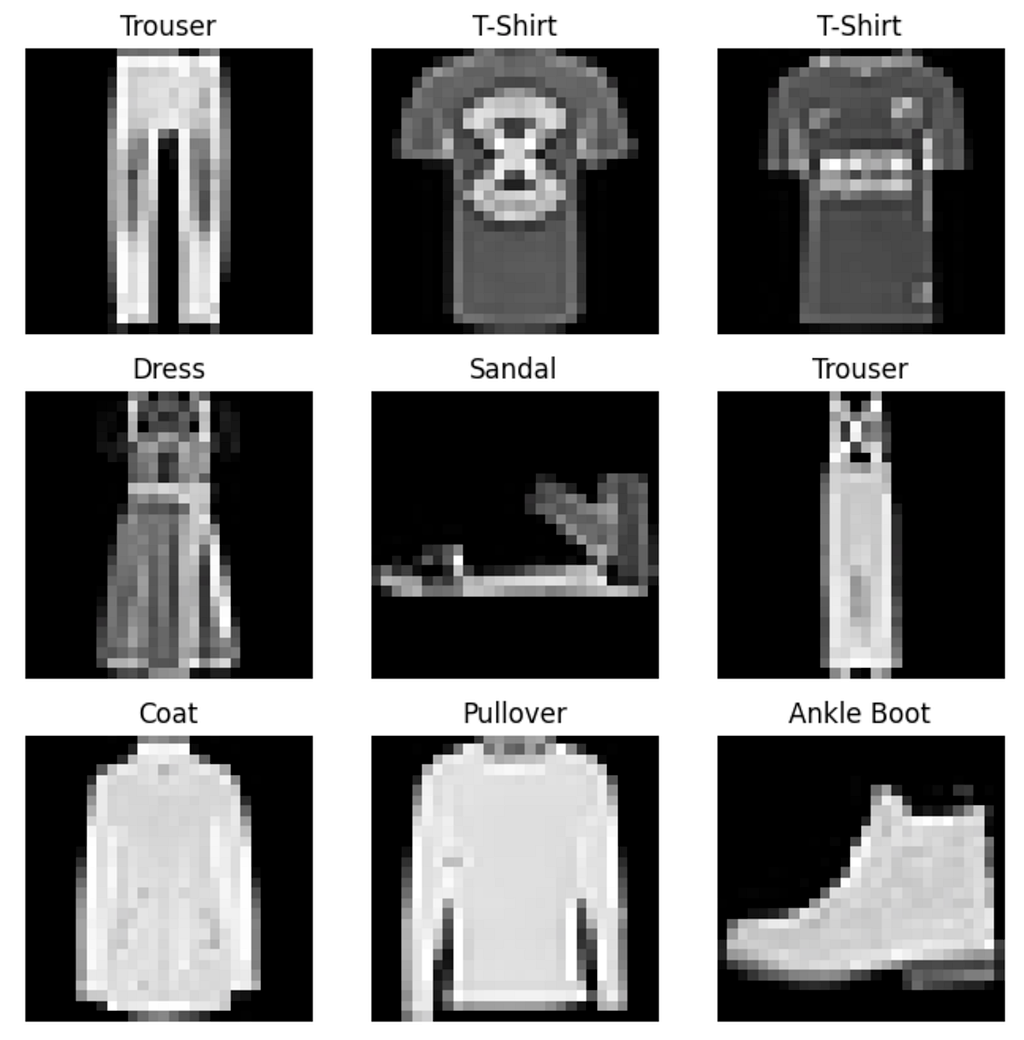
Can a large pretrained vision model perform well on a small, low-resolution fashion dataset without training on every available example? I used a pretrained Vision Transformer, limited training to 6,000 Fashion-MNIST images because of local compute constraints, and implemented the training loop directly in PyTorch.
Experiment snapshot
- Question: How effectively can a pretrained ViT adapt to Fashion-MNIST with limited training data?
- Constraint: Train on 6,000 of the 60,000 available training images.
- Result: Macro F1 of 0.9318 on held-out data.
- Artifact: Run the notebook on Kaggle.
The interesting parts are the boundaries between tools: reshaping Fashion-MNIST for the model, replacing the classifier head, running gradient descent without a high-level trainer, and evaluating more than raw accuracy.
Background
Fashion-MNIST contains 60,000 training images and 10,000 test images across ten clothing categories. Each source image is only 28×28 pixels and grayscale.
The starting checkpoint is google/vit-base-patch16-224. It was pretrained on ImageNet-21k and then fine-tuned on the 1,000-class ImageNet-1k task at a resolution of 224×224. Its existing classification head therefore produces 1,000 outputs; Fashion-MNIST needs only ten.
Transfer learning lets us preserve the useful visual representations learned by the transformer while replacing that final task-specific layer.
Load the data
Hugging Face Datasets makes the source data available with a single call:
from datasets import load_dataset

raw_dataset = load_dataset("zalando-datasets/fashion_mnist")
The result already contains the expected training and test splits:
DatasetDict({
    train: Dataset({
        features: ['image', 'label'],
        num_rows: 60000
    })
    test: Dataset({
        features: ['image', 'label'],
        num_rows: 10000
    })
})
The local machine used for the experiment could not comfortably train ViT on all 60,000 images, so I deliberately used a 6,000-image subset:
from datasets import Dataset

train_dataset = Dataset.from_dict(raw_dataset["train"][:6000])
That constraint made the experiment more interesting: the base model had to contribute meaningful prior knowledge rather than relying on the full training set.
Process the inputs
The source images do not match the checkpoint. Fashion-MNIST images are 28×28 grayscale; ViT expects normalized 224×224 RGB inputs. The checkpoint’s image processor handles the conversion consistently:
from transformers import AutoImageProcessor

checkpoint = "google/vit-base-patch16-224"
image_processor = AutoImageProcessor.from_pretrained(checkpoint)

def preprocess_images(examples):
    images = [image.convert("RGB") for image in examples["image"]]
    inputs = image_processor(images=images, return_tensors="pt")
    examples["pixel_values"] = inputs["pixel_values"]
    return examples
Testing two examples confirms the tensor shape:
processed = preprocess_images(raw_dataset["train"][0:2])
print(processed["pixel_values"].shape)

# torch.Size([2, 3, 224, 224])
The first dimension is the batch size, the second contains the three RGB channels, and the last two are the resized image dimensions. Upscaling does not create new image detail, but it places the data in the shape and normalization regime expected by the pretrained model.
Replace the classification head
The checkpoint’s classifier produces 1,000 ImageNet labels. Passing num_labels=10 and allowing mismatched sizes tells Transformers to retain the encoder weights while initializing a new ten-class head:
from transformers import AutoModelForImageClassification

model = AutoModelForImageClassification.from_pretrained(
    checkpoint,
    num_labels=len(labels_map),
    ignore_mismatched_sizes=True,
)
The warning produced here is expected:
classifier.bias:   found shape [1000], expected [10]
classifier.weight: found shape [1000, 768], expected [10, 768]
The new head starts untrained. It must learn how the encoder’s visual representation maps to Fashion-MNIST’s ten categories.
Train with PyTorch
High-level trainers could hide most of the loop, but this experiment was partly about understanding the mechanics. Each batch moves to the available device, passes through the model, calculates loss, backpropagates gradients, updates the weights, advances the learning-rate schedule, and clears the gradients before the next batch.
for epoch in range(num_epochs):
    for batch in train_dataloader:
        batch = {key: value.to(device) for key, value in batch.items()}

        outputs = model(**batch)
        loss = outputs.loss

        loss.backward()
        optimizer.step()
        lr_scheduler.step()
        optimizer.zero_grad()
Writing this explicitly makes the state changes visible. It also makes it harder to forget details—especially clearing accumulated gradients—that a higher-level abstraction normally handles.
Evaluate the model
Accuracy alone can conceal uneven performance across classes. I combined macro-averaged F1, precision, and recall so every clothing category contributed equally to the aggregate metrics:
import evaluate

classification_metrics = evaluate.combine(["f1", "precision", "recall"])

results = classification_metrics.compute(
    predictions=all_predictions,
    references=all_references,
    average="macro",
)

print(f"F1 Score:  {results['f1']:.4f}")
print(f"Precision: {results['precision']:.4f}")
print(f"Recall:    {results['recall']:.4f}")
F1 Score:  0.9318
Precision: 0.9329
Recall:    0.9317
The three values are both high and tightly grouped. In this run, the classifier maintained a good balance between false positives and false negatives across the ten categories despite using only a tenth of the available training images.
What the result does—and does not—show
The result is a strong demonstration of transfer learning: a model with useful pretrained visual representations adapted to a new ten-class task with relatively little data.
It is not proof that this is the best Fashion-MNIST architecture. The experiment did not include a systematic hyperparameter sweep, multiple random seeds, calibration analysis, per-class error analysis, or a comparison against a smaller convolutional baseline. ViT is also much larger than necessary for this dataset, and resizing 28×28 images to 224×224 adds compute without adding visual information.
A useful next iteration would compare the model against a compact CNN, examine the confusion matrix, train across several seeds, and measure whether the extra model size buys enough improvement to justify its cost.