I wanted to know whether a compact pretrained vision model could clear 90% accuracy on CIFAR-10 without training a network from scratch. I adapted MobileNetV2 in two phases: first training a new classification head while keeping the pretrained backbone frozen, then fine-tuning part of that backbone with a smaller learning rate.
The saved confusion matrix shows 91.78% accuracy across 10,000 images, with training accuracy around 93%. The result showed that transfer learning could adapt a relatively small model to low-resolution images, but the error analysis also exposed a persistent weakness: cats were often classified as dogs.
This is the first part of the experiment. Transfer Learning II compares this hand-built model with Vertex AI AutoML.
Experiment snapshot
- Question: Can MobileNetV2 exceed 90% accuracy on CIFAR-10 through transfer learning?
- Dataset: CIFAR-10, with 60,000 32×32 color images across ten classes.
- Approach: Train a new ten-class output head, then fine-tune the later MobileNetV2 layers.
- Result: 91.78% accuracy in the saved 10,000-image confusion matrix, compared with roughly 93% training accuracy.
- Artifact: Open the manual-model notebook in Google Colab.
- Main limitation: The experiment used a single model run and did not systematically compare fine-tuning boundaries, augmentation strategies, or alternative architectures.
Why transfer learning
Deep-learning models can require substantial data and compute when trained from scratch. Transfer learning starts from a model that has already learned useful visual features on a larger dataset and adapts those features to a new task.
MobileNetV2 was a practical starting point because it was designed to balance image-classification accuracy with a small computational footprint. Its ImageNet-trained backbone already recognized general patterns such as edges, textures, and shapes. My task was to replace its original classifier with one that could distinguish CIFAR-10’s ten categories: airplane, automobile, bird, cat, deer, dog, frog, horse, ship, and truck.
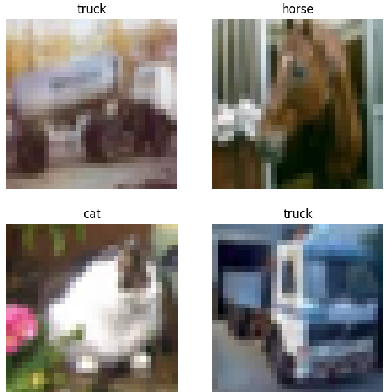
The 32×32 source images are challenging even for a person. In the sample above, the cat is not immediately obvious. That low resolution shaped the two-stage training strategy.
Phase 1: Train the classification head
I first removed MobileNetV2’s original ImageNet classification layer, froze the pretrained backbone, and added a ten-neuron softmax layer. Freezing the backbone meant that training changed only the new task-specific head.
base_model = tf.keras.applications.MobileNetV2(
    include_top=False,
    input_shape=(32, 32, 3),
    name="warmup_checkpoint",
    weights="imagenet",
)
base_model.trainable = False

model = tf.keras.Sequential([
    tf.keras.layers.Input(shape=(32, 32, 3)),
    # Preprocessing steps omitted for brevity.
    base_model,
    tf.keras.layers.GlobalAveragePooling2D(),
    tf.keras.layers.Dense(10, activation="softmax"),
])

model.compile(...)
model.fit(...)
model.save("warmup_checkpoint.keras")
This first phase reached roughly 82% validation accuracy. More importantly, it created a checkpoint with a trained CIFAR-10 head that I could refine without immediately disturbing the pretrained features.
Phase 2: Fine-tune the backbone
Feature extraction leaves the backbone untouched. Fine-tuning allows some of its weights to change so the later features can better represent the new dataset.
The boundary matters. Unfreezing too much of the network can overwrite useful pretrained representations, a failure mode called catastrophic forgetting. Keeping every layer frozen, however, limits the model’s ability to adjust to CIFAR-10’s unusually small and blurry images.
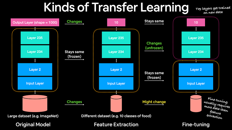
Diagram adapted from Daniel Bourke’s transfer-learning material.
For this run, I loaded the warm-up checkpoint, made the MobileNetV2 backbone trainable, then kept the layers before index 110 frozen. That left the later portion of the roughly 154-layer backbone available for fine-tuning. I also reduced the learning rate so each update would make a relatively small change to the pretrained weights.
model_finetuned = tf.keras.models.load_model(
    "warmup_checkpoint.keras"
)

layer_container = model_finetuned.get_layer("warmup_checkpoint")
layer_container.trainable = True

for layer in layer_container.layers[:110]:
    layer.trainable = False

model_finetuned.compile(
    loss="sparse_categorical_crossentropy",
    optimizer=tf.keras.optimizers.Adam(learning_rate=...),
    metrics=["accuracy"],
)

hist_fine = model_finetuned.fit(...)
This distinction is easy to miss: the implementation did not fine-tune only five or ten layers. Freezing through layer 110 left roughly 44 MobileNetV2 layers trainable, although some of those layers may not contain learned parameters.
Evaluate the errors
The aggregate score met the original goal, but the confusion matrix made the remaining failure modes more useful to inspect.
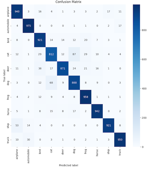
Cats were the weakest class in this evaluation. Of the 1,000 cat images represented in the matrix, 812 were classified correctly and 87 were labeled as dogs. The reverse confusion was also visible: 68 dog images were labeled as cats.
The matrix contains 9,178 correct predictions out of 10,000, or 91.78% accuracy. This is separate from the shared 600-image evaluation in Transfer Learning II, which compares F1 scores. Accuracy and F1 measure different things, and the two evaluations should not be treated as the same result.
Data augmentation or a different fine-tuning boundary could improve the cat-versus-dog errors. A stronger follow-up would test those changes across multiple seeds and compare the results against a smaller convolutional baseline.
What this established
The feature-extraction phase reached roughly 82% validation accuracy; after fine-tuning, the model reached 91.78% accuracy on a 10,000-image evaluation. This was one model run, and the result alone does not establish how well the model generalizes beyond this dataset.
The more practical question is whether this result justified the engineering work. Transfer Learning II runs the same classification problem through Vertex AI AutoML and compares the outcome.